Interactive Cell Tracking with Napari Track Edit

September 2026 - Napari Track Edit v1.* - Caroline Malin-Mayor - Teun Huijben - Anniek Stokkermans

Napari Track Edit is a Napari plugin for interactive visualization, navigation, and editing of object tracking results. You can open and edit existing tracking data, manually create new tracking results, or run automatic tracking via the Napari Track Edit integration, which offers object tracking using the motile library.

This tutorial will walk you through the main functionalities. You can find the full documentation here.

Preparations

Installation

You can install the plugin via pypi in the environment of you choice (e.g. venv, conda) with the command pip install napari-track-edit. Currently, this requires python >=3.11.

For example, to create a new environment with conda:

conda create -n napari_track_edit python=3.12
conda activate napari_track_edit
pip install "napari-track-edit[all]"

Verify installation of the plugin

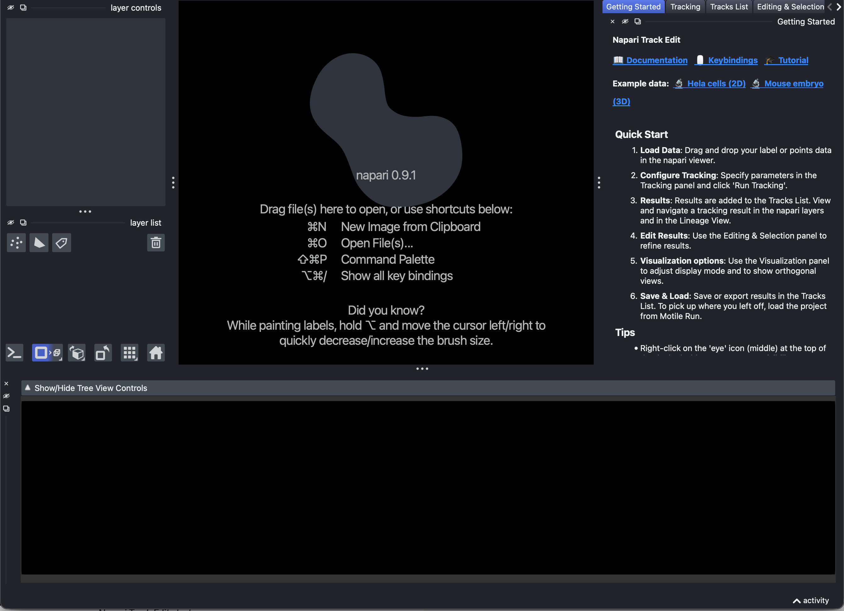
If your installation was successful, you should be able to start napari from the terminal and find ‘Napari Track Edit’ under Plugins. Please go to Plugins > Napari Track Edit > Open all widgets to check if the start up screen looks like this:

Downloading sample data

Two sample datasets are provided with the plugin:

Fluo-N2DL-HeLa is a 2D dataset of images and segmentations of HeLa cells from the cell tracking challenge.
Mouse Embryo Membrane is a 3D dataset of images and segmentations of a membrane labeled developing early mouse embryo (4-26 cells) from Fabrèges et al (2024) available here.

The sample image data are listed under File > Open Sample > Napari Track Edit > Fluo-N2DL-HeLa (2D) and File > Open Sample > Napari Track Edit > Mouse Embryo Membranes (3D). Tracks for the sample data are available as well: go to Plugins > Napari Track Edit > Getting Started, and click on one of the two examples: Hela cells (2D) or Mouse embryo (3D) to download and view them. After downloading, the data will remain available in the plugin for re-use.

Plugin layout

All plugin widgets are listed under Plugins > Napari Track Edit, where they can be (re)opened individually or all at once. You can hide, close, or rearrange the widgets as you like. The / key toggles the visibility of all widgets at once. You can find an overview of all mouse and keyboard bindings at the end of this document.

Inspecting a tracking result

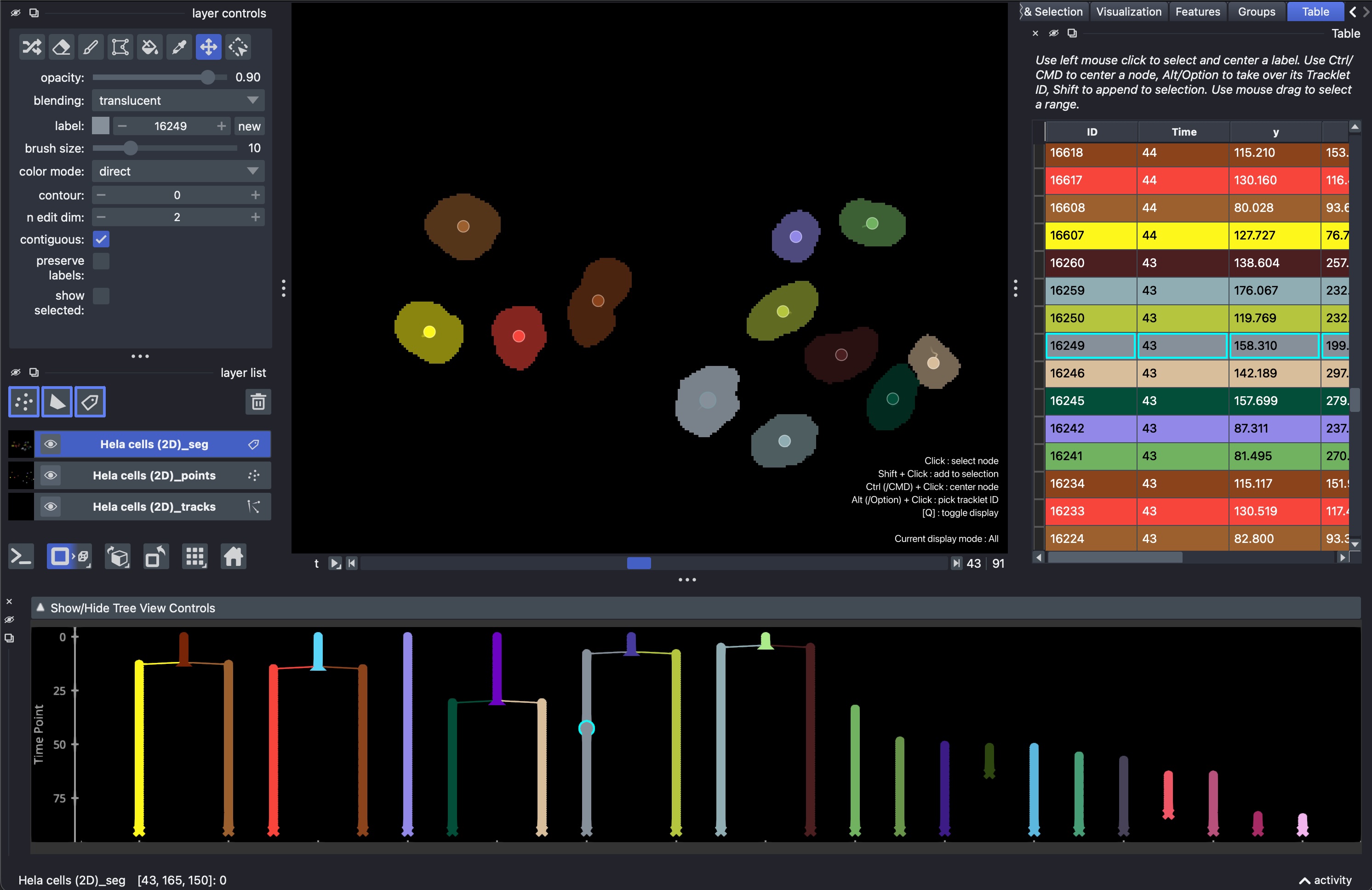
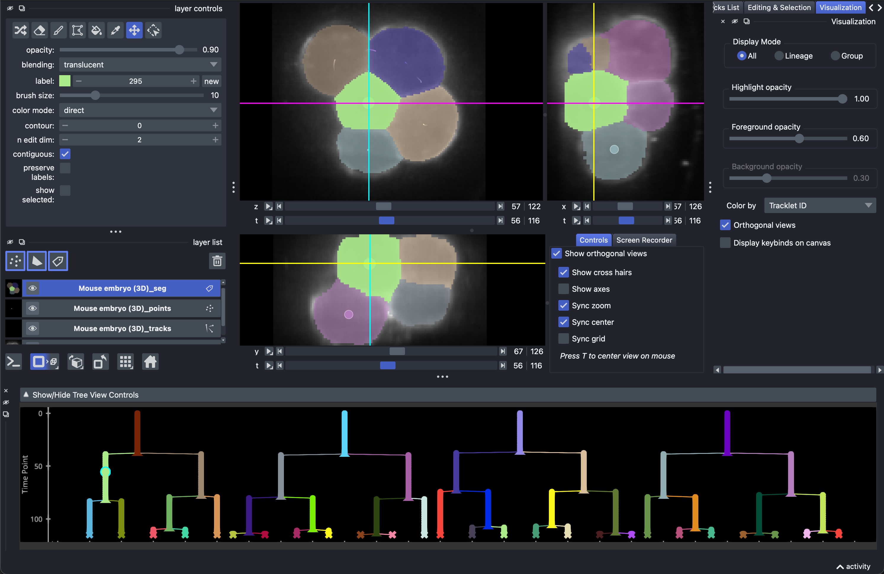
To get familiar with the tool, it is easiest to look at an example first. Opening the sample data via Plugins > Napari Track Edit > Getting Started should look like this:

Viewing HeLa Cells (2D) sample tracks with the Table widget active

Viewing Mouse Embryo (3D) sample tracks with orthogonal views enabled

Track visualization

Tracking results are displayed with:

a Points layer, with nodes color-coded by tracklet ID and with symbols matching the state of the node:
- △ dividing node
- ✕ end point node
- ◯ linear node
an optional Segmentation (Labels) layer, with label values matching node ids, but color-coded by tracklet ID
a Tracks layer, with tracks color-coded by tracklet ID
a Lineage View, available from Plugins > Napari Track Edit > Widget - Lineage View, with nodes and edges color-coded by tracklet ID and with symbols matching the state of nodes.
a Table View, available from Plugins > Napari Track Edit > Widget - Table, with all object properties.

Selecting nodes

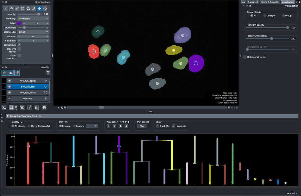
You can select one or multiple nodes for closer inspection. Selection of nodes is possible in the Points and Labels layers, in the Lineage View, and in the Table view. Selecting a single node highlights it and centers the object if it is outside the viewing range. You can append (or subtract) nodes to (from) the selection by pressing SHIFT when clicking. You can restrict the display to the lineages of selected nodes in the Viewer (via the Visualization tab) and in the Lineage View (via the Lineage View controls).

Display the lineages that have at least one selected node

Exercise 1 - View and explore a tracking result

1. Go to the Getting Started widget and open one of the two examples. Also open the Lineage View and Table widgets.

2. Inspect the tracks in the Napari Viewer, the Lineage View, and in the Table widget. You can click in any of these views to select and center nodes and use scroll to zoom in to specific regions. Use right-mouse click to reset the Lineage View.

3. Try selecting multiple nodes with SHIFT+CLICK or SHIFT+DRAG (in the Lineage View and Points layer, with the 'select points'-tool active).

4. Open the Editing & Selection widget and look at the 'Selection' section. Test the buttons and keyboard shortcuts to clear, restore, and cycle through selections.

5. Hover over nodes in the Lineage View and inspect the information you can read there. What is the difference between a Track and a Lineage?

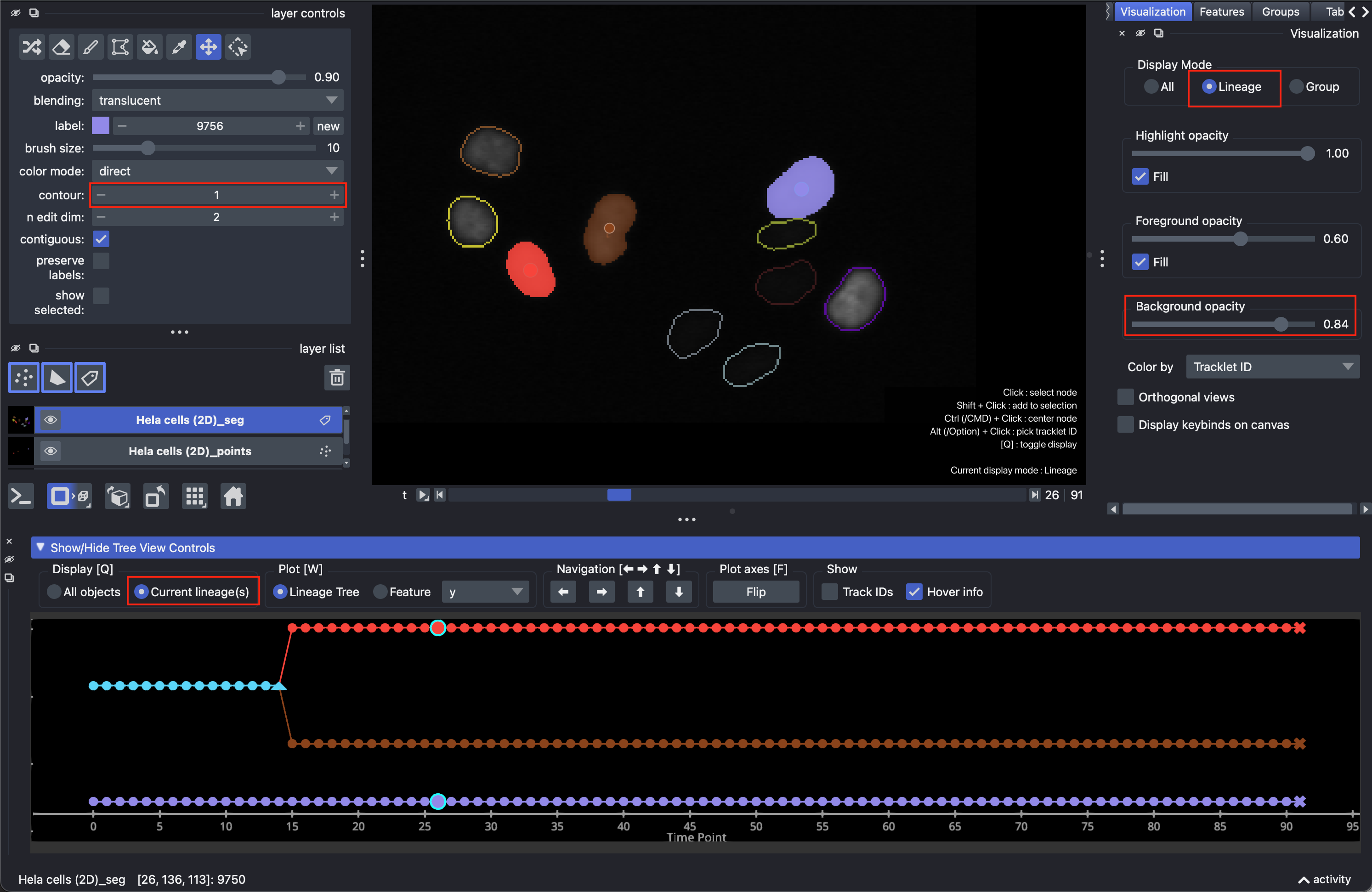
6. Open the Visualization tab and switch the Display Mode to 'Lineage'. What happens to the labels? Try the different sliders for 'highlight', 'foreground', and 'background' opacity, do you understand what they each refer to? What happens if you set the 'contour' value to 1 in the layer controls (top left menu)?

7. Open the Lineage View controls and set the display mode to 'Current lineage(s)', and change your selection by clicking on different nodes in the Viewer. Try out the arrow buttons or arrow keys to move up or down the tree or to jump to neighboring nodes.

8. If you had loaded the 3D example, go back to the Visualization widget, and activate the orthogonal views. Try out the settings in the OrthoView control widget. Press T to center all views on your mouse cursor. You can also do this for the 2D example, but you will see the time axis in the ortho views instead.

Generating Tracks

There are two ways to obtain a new tracking result from within the plugin: manual tracking on an image layer, or automatic tracking using Motile on a Labels or Points layer. We will explore both methods here.

Manual tracking

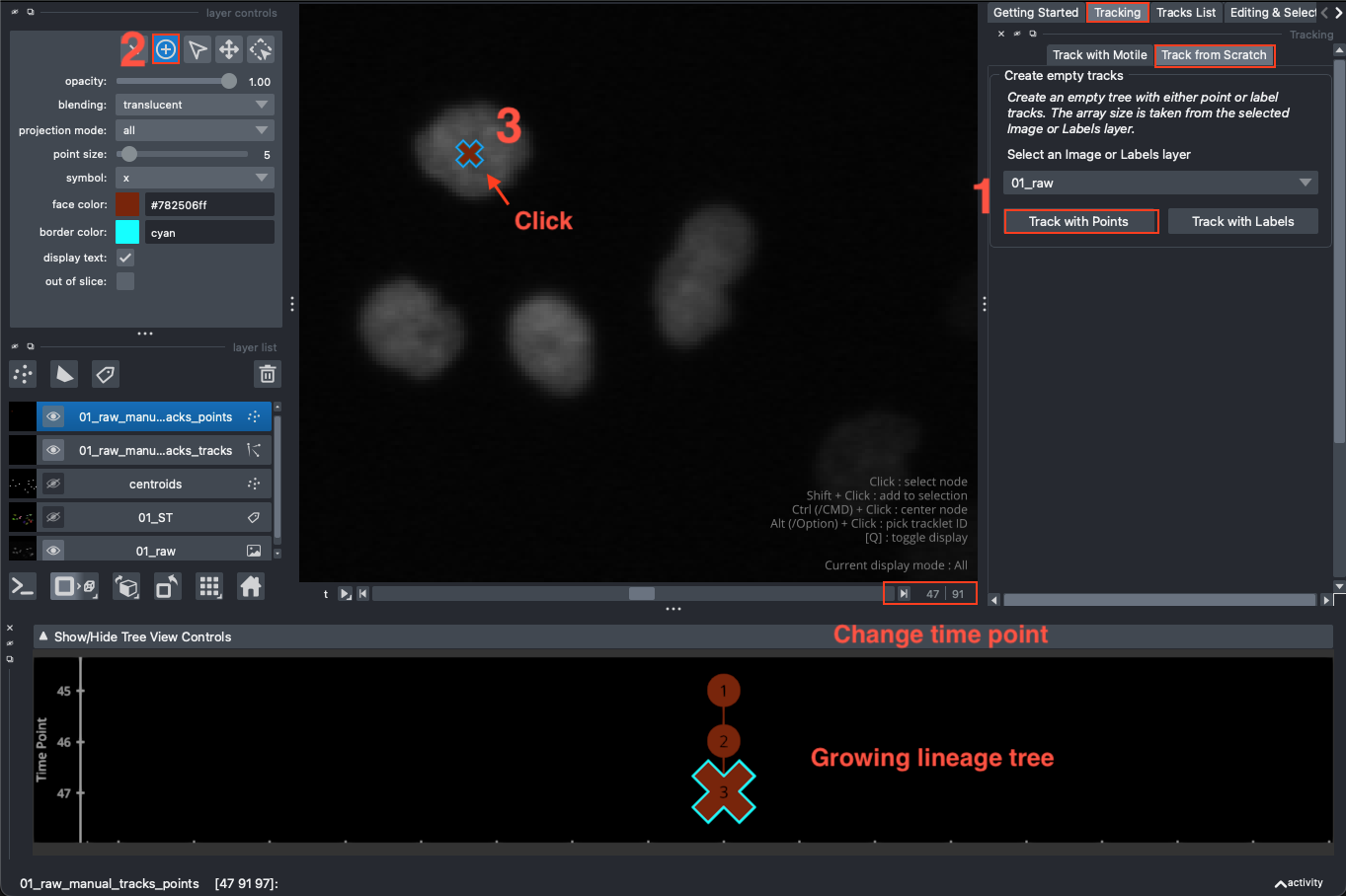
Manual tracking from scratch requires that you open an Image layer first. In the Tracking widget, under Track from Scratch you can select this layer, and choose to either Track with Points or Track with Labels. Depending on your choice, this will create either an empty Points or empty Labels layer, where you can manually add points or paint labels to track objects.

Tracking with Motile

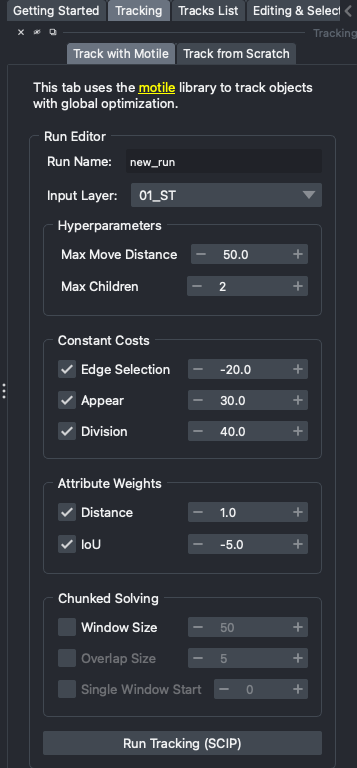
To track objects with Motile, you need to either provide object segmentations on a Napari Labels layer or object detections on a Points layer. Tracking parameters should be specified in the Tracking > Track with Motile tab and are subdivided in hyperparameters, constant costs and attribute weights. Hovering over each of the parameters will display a tooltip, and more extensive information can be found in the documentation. Once the parameters are set, you can start the solver by clicking Run Tracking. 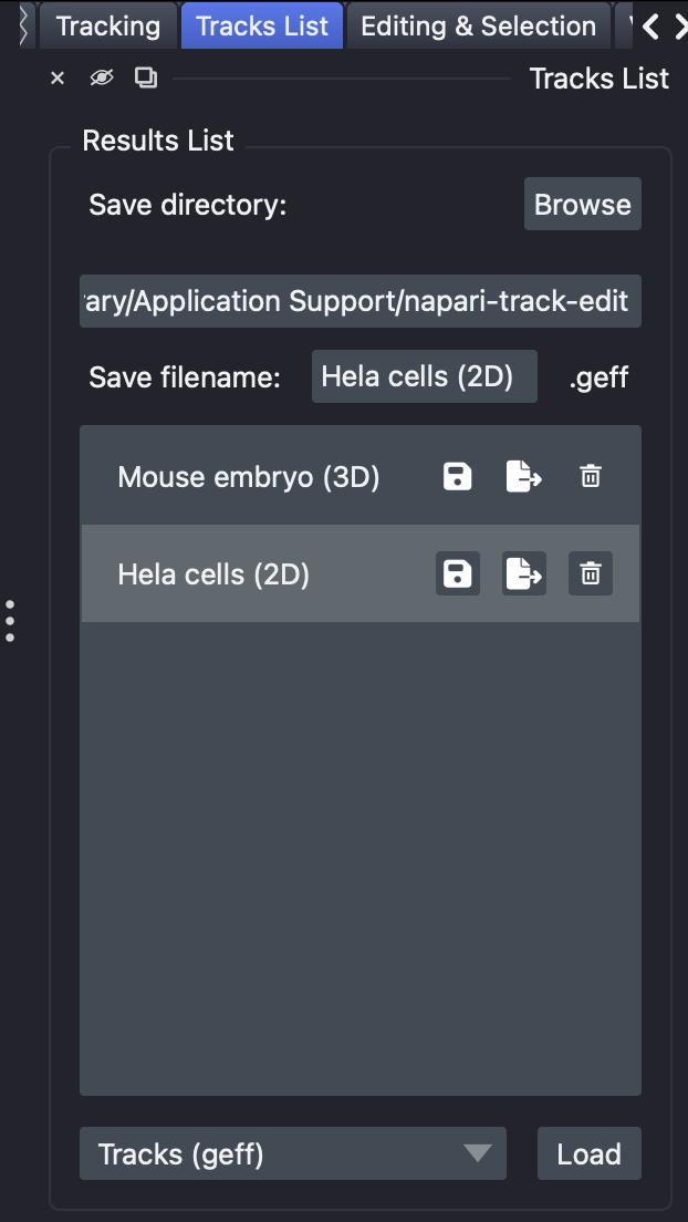After the solve is complete, you can find the Tracking Result in the Tracks List tab. Tracking Results will accumulate here for each set of parameters that you tried.

Exercise 2 - Generating new tracks

1. Go to the Tracks List tab first, and clear the example tracks by clicking on the trash can icon.

2. Go to File > Open Sample > Napari Track Edit > Fluo-N2DL-HeLa crop (2D) to open the 2D HeLa cell test dataset

3. Hide the segmentation '01_ST' and 'centroids' layers for now, but select 01_raw and go to the Tracking > Track from Scratch. Select 01_raw from the dropdown menu, and click Track with Points. A new Points layer is generated, and you should see a new element in the Results list: 01_raw_manual_tracks. Select the Add points tool in the top left corner of the layer controls, and click on one of the nuclei in the viewer. Go to the next time point, and click again. You should see a growing lineage tree at the bottom of your screen. What happens if you add multiple points in the same time point? Try to build three small lineages.

4. To compute tracks automatically, go to the Tracking tab, and choose parameters for tracking. Use '01_ST' as input layer. You can consult the documentation to help you decide on the different values. Click Run Tracking to start the computation. After the solver has finished, you should see that the Lineage View is now populated with tracks and that the cells are relabeled.

5. Click Back to editing and test multiple combinations of parameters. Note that you can also use the Points layer 'centroids' as input. Compare the different tracking results by clicking on the different entries in the Tracks List widget.

Displaying object features in the Lineage View

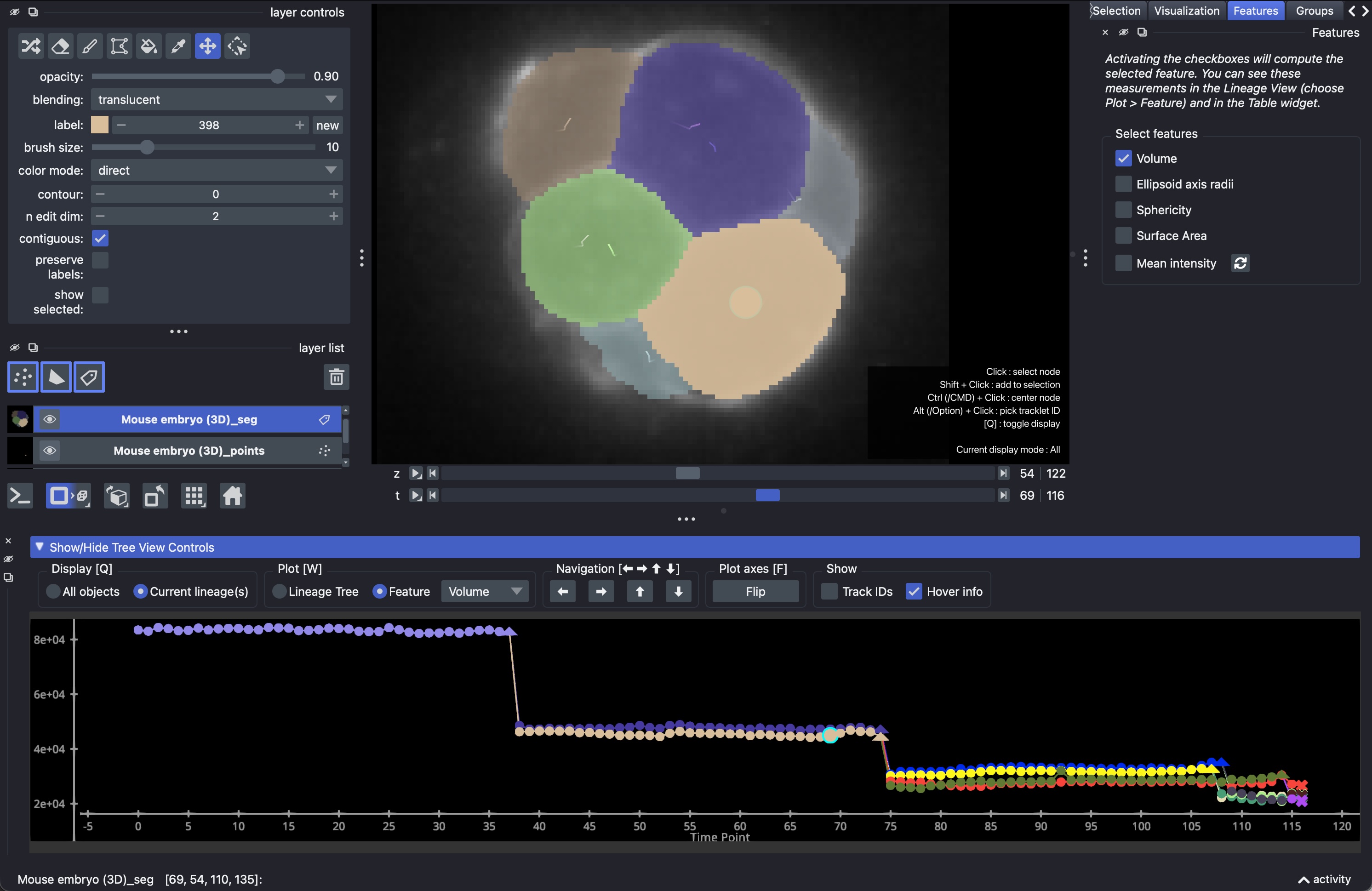
Apart from the lineage tree, you can also view object properties in the Lineage View. The Feature widget displays a list of size, shape, and intensity features that you can activate. All activated features will appear as columns in the Table widget and in the ‘Feature’ dropdown menu in the Lineage View controls. To display a feature, activate the ‘Feature’ radio button and select a feature from the list.

Creating groups

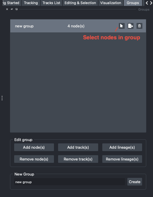
In the Groups tab you can create groups of nodes that you want to store to review later, for example because these are of particular interest, need to be corrected, or belong to a specific object/cell type. You can add or remove individual nodes, entire tracks, or entire lineages. You can also select all nodes in a group or export them.

Exercise 3 - Measure features and create groups

1. Open the Features widget and activate one or multiple features. Note that this is only possible if you are currently viewing a tracking result that has an associated Labels layer, because most features, like size, cannot be computed for Points. Switch to 'Feature' in the Lineage View controls and display a feature of your choice. You may want to switch to viewing selected lineages to make the plot less crowded.

2. Verify that you can also find these measurements back in the Table widget. Try deactivating and activating different features and check the measurements in the table.

3. Open the Groups widget and make a new group. Sort the Table widget by Area (or Volume) by clicking on the header and select the top 10 rows and add these nodes to a group. Verify that you can always go back to select the nodes in this group by clicking on the mouse pointer button.

4. Create another group and test the 'edit group' buttons. Verify that you can restrict the display to the nodes in the group by changing the display mode to 'group' in the Visualization widget.

Editing Tracks

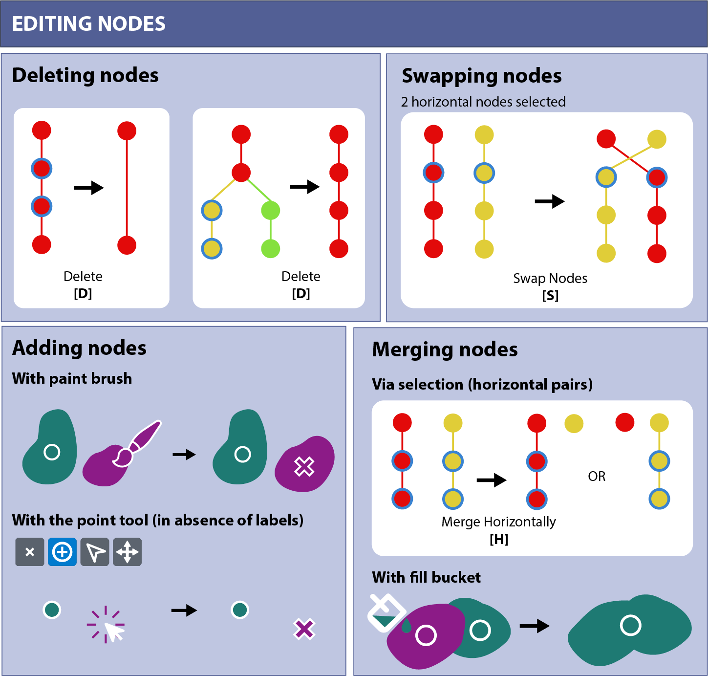
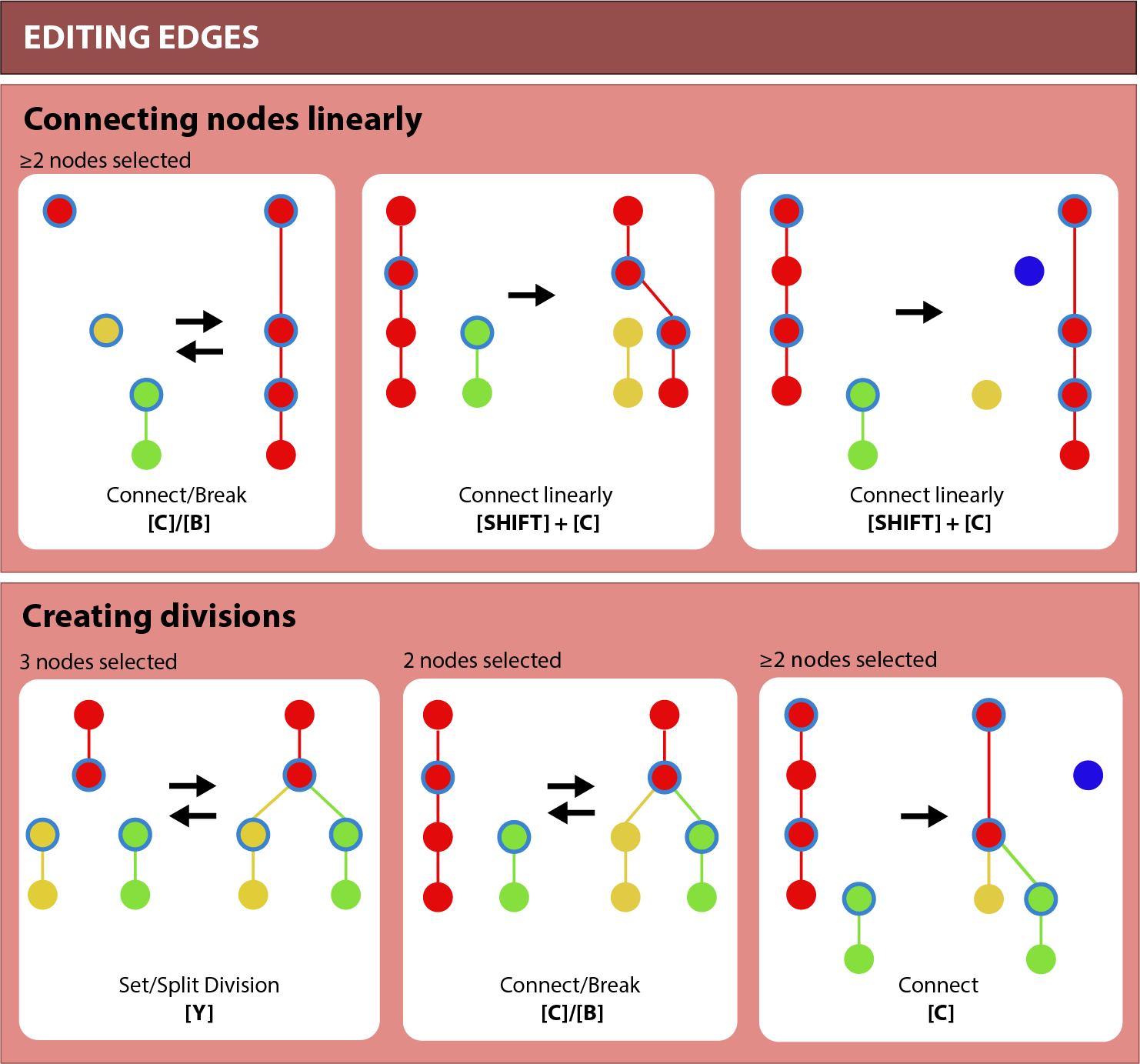
When inspecting a tracking result, you may notice mistakes that you want to correct by deleting, adding, or modifying nodes and/or edges. You can edit the tracks using the buttons in the Editing & Selection tab or their corresponding keyboard shortcuts, or by editing the Napari Points and Segmentation layers directly. To undo/redo an action, click Undo/Redo in the menu or press Z/ R. Find out more in documentation.

Exercise 4 - Editing tracks

1. Open the Editing & Selection widget.

2. Select one or multiple nodes, and use the Delete button or press D to delete them. What happens if you:

delete a linear node?
delete a dividing node?
delete an end point node?
delete one of the two children of a dividing node?

You can undo your actions by pressing Z or with the Undo button.

3. Go to the Segmentation layer ('_seg') and activate the paint brush. Press M to select a new label. Paint a new node and observe the Lineage View. Then move to the next time point and paint with the same color again. Observe that a new track is created as you are painting.

4. Select a new node and display the object size in the Lineage View. Then paint or erase part of it in the Segmentation layer. Observe how this affects the object size and the centroid location.

5. Select two connected nodes and use the Break button or press B to break the connection. What happens to the two fragments?

6. Select two nodes and try to create an edge between them with the Connect button or by pressing C. Try to answer these questions:

Can you connect any two nodes?
What happens if there is a time gap between the two nodes?
Can you connect more than two nodes in one go?
What happens if you connect to a node that already has an outgoing edge to another node?
What happens if the node your are connecting to already has an incoming edge?

7. Select two nodes in the same time point in the Napari Viewer, and press S to swap the predecessors of those nodes, assigning them to each other's tracklet IDs. Does the tree view change?

8. Select two nodes in the same time point, and press H to merge them into one node with the Tracklet ID of your choice.

9. Select a trio of nodes: two at the same time point and one at the time point before, and press Y to set a division here. Press Y again to break the division.

Saving and reopening Tracks

You can save your tracking results in the Tracks List tab. This will save the parameters and the tracking data to the displayed destination. You can load your results back in at the bottom of the Tracks List tab by loading a Motile Run and selecting the folder. In addition, Napari Track Edit allows you to import and export the results from/to csv and geff via the dropdown menu at the bottom and the export (middle) button in the Results List.

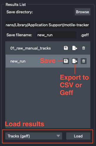
Exercise 5 - Save and load tracking results

1. Go to the Tracks List tab.

2. Select a save directory on your computer via the Browse button, and click the save button to save the tracks.

3. Click the trash can icon to delete the tracks from the list.

4. At the bottom of the Tracks List tab, choose Motile Run from the dropdown menu to load your saved tracks back into the plugin.

5. Export your tracking results to csv with the export button in the Results List (next to the save and trash buttons). You will be asked whether to include saving the segmentation (as-is or relabeled by tracklet ID).

7. At the bottom of the Tracks List tab, choose External Tracks from CSV from the dropdown menu to load the results back from the csv file. If you have a segmentation image, you must provide a segmentation id, which corresponds to the label value for each node in the segmentation image (if you exported with 'Relabel segmentation by Track ID', this value should be set to Tracklet ID).

8. Export your tracking result to geff. Note that the segmentation data is included in the geff, so you do not need to save it separately.

9. Load the geff via External Tracks from geff.

10. Go to the Groups widget, and export a group to csv and inspect the file. Which nodes are included when you load it back in?

Mouse and keyboard bindings

Shortcuts work in the napari viewer (with a tracks layer selected), the Lineage View and the Table (click on it first to give it focus). Nodes can be clicked as points or labels in the viewer, as nodes in the Lineage View, and as rows in the Table (drag to select a range).

Selection

Key / mouse	Action
Click on a node	Select this node (centers the view on it if it is the only selected node)
`Shift` + click	Add/remove this node to/from the selection
`Ctrl`/`Cmd` + click	Center the view on this node, without changing the selection
`Alt`/`Option` + click	Make this node’s tracklet ID the current one, without changing the selection or time point
Mouse drag	Select multiple nodes: ‘select points’ tool (Points layer), `Shift` + drag (Lineage View)
`Esc`	Clear the selection
`E`	Restore the last selection
`P` / mouse back	Select the previous node set from the selection history
`N` / mouse forward	Select the next node set from the selection history

Editing

Key	Action
`M`	Start a new track: assign a new track id, and a new segmentation label if necessary
`D` or `Del`	Delete the selected nodes
`S`	Swap the incoming edges of two nodes at the same time point
`C`	Connect the selected nodes into one track, keeping existing outgoing edges as divisions
`Shift` + `C`	Connect the selected nodes into one linear track, breaking existing outgoing edges
`B`	Break the edges between the selected nodes (edges to other nodes are kept)
`Y`	Make or break a division between a parent node and its two children
`H`	Merge each set of selected nodes that shares a time point into a single node
`Z`	Undo the last editing action
`R`	Redo the last undone editing action

View

Key / mouse	Action
`/`	Hide or show all currently active widgets
`Q`	Cycle the display mode: All → Lineage → Group (Group only when groups exist)
`T`	Center the orthogonal views on the mouse cursor
Click column header	Sort the Table by this column

Lineage view

Key / mouse	Action
`Q`	Switch between all lineages and the selected lineages
`W`	Switch the lineage view between the tree plot and a feature plot
`F`	Flip the axes of the lineage view
`←` / `→`	Select the node to the left / right
`↑` / `↓`	Select the parent / child node, or the next / previous lineage (selected lineages view)
Scroll (+ `X` / `Y`)	Zoom in or out (only along the x / y axis)
Right drag	Stretch or squeeze the axes (horizontally: x axis, vertically: y axis)
Mouse drag	Pan
Right click	Reset the view

Thank you for participating in the workshop!